import pandas as pd
import numpy as np

import matplotlib.pyplot as plt
from matplotlib import gridspec
from matplotlib.offsetbox import (OffsetImage, AnnotationBbox)

import mathExploratory Data Analysis of Song Data
Song data comes from the top singles list for each year from 1958 to 2022.
Data features are gathered from the Spotify API (here)[https://developer.spotify.com/documentation/web-api/reference/#/operations/get-audio-features].
plt.plot();
plt.style.use("datafantic-right.mplstyle")df = pd.read_csv("songs.csv")df| entry_date | title | artist | peak | peak_date | weeks_top_ten | year | spotify_uri | danceability | energy | ... | liveness | valence | tempo | type | id | uri | track_href | analysis_url | duration_ms | time_signature | |
|---|---|---|---|---|---|---|---|---|---|---|---|---|---|---|---|---|---|---|---|---|---|
| 0 | August 4 | "Poor Little Fool" | Ricky Nelson | 1 | August 4 | 6 | 1958 | spotify:track:5ayybTSXNwcarDtxQKqvWX | 0.474 | 0.338 | ... | 0.1300 | 0.8100 | 154.596 | audio_features | 5ayybTSXNwcarDtxQKqvWX | spotify:track:5ayybTSXNwcarDtxQKqvWX | https://api.spotify.com/v1/tracks/5ayybTSXNwca... | https://api.spotify.com/v1/audio-analysis/5ayy... | 153933.0 | 4.0 |
| 1 | August 4 | "Patricia" | Pérez Prado | 2 | August 4 | 6 | 1958 | spotify:track:2bwhOdCOLgQ8v6xStAqnju | 0.699 | 0.715 | ... | 0.0704 | 0.8100 | 137.373 | audio_features | 2bwhOdCOLgQ8v6xStAqnju | spotify:track:2bwhOdCOLgQ8v6xStAqnju | https://api.spotify.com/v1/tracks/2bwhOdCOLgQ8... | https://api.spotify.com/v1/audio-analysis/2bwh... | 140000.0 | 4.0 |
| 2 | August 4 | "Splish Splash" | Bobby Darin | 3 | August 4 | 3 | 1958 | spotify:track:40fD7ct05FvQHLdQTgJelG | 0.645 | 0.943 | ... | 0.3700 | 0.9650 | 147.768 | audio_features | 40fD7ct05FvQHLdQTgJelG | spotify:track:40fD7ct05FvQHLdQTgJelG | https://api.spotify.com/v1/tracks/40fD7ct05FvQ... | https://api.spotify.com/v1/audio-analysis/40fD... | 131720.0 | 4.0 |
| 3 | August 4 | "Hard Headed Woman" | Elvis Presley | 4 | August 4 | 2 | 1958 | spotify:track:3SU1TXJtAsf8jCKdUeYy53 | 0.616 | 0.877 | ... | 0.1840 | 0.9190 | 97.757 | audio_features | 3SU1TXJtAsf8jCKdUeYy53 | spotify:track:3SU1TXJtAsf8jCKdUeYy53 | https://api.spotify.com/v1/tracks/3SU1TXJtAsf8... | https://api.spotify.com/v1/audio-analysis/3SU1... | 114240.0 | 4.0 |
| 4 | August 4 | "When" | Kalin Twins | 5 | August 4 | 5 | 1958 | spotify:track:3HZJ9BLBpDya4p71VfXSWp | 0.666 | 0.468 | ... | 0.1190 | 0.9460 | 93.018 | audio_features | 3HZJ9BLBpDya4p71VfXSWp | spotify:track:3HZJ9BLBpDya4p71VfXSWp | https://api.spotify.com/v1/tracks/3HZJ9BLBpDya... | https://api.spotify.com/v1/audio-analysis/3HZJ... | 146573.0 | 4.0 |
| ... | ... | ... | ... | ... | ... | ... | ... | ... | ... | ... | ... | ... | ... | ... | ... | ... | ... | ... | ... | ... | ... |
| 4246 | June 4 | "Matilda" | Harry Styles | 9 | June 4 | 1 | 2022 | spotify:track:6uvh0In7u1Xn4HgxOfAn8O | 0.507 | 0.294 | ... | 0.0966 | 0.3860 | 114.199 | audio_features | 6uvh0In7u1Xn4HgxOfAn8O | spotify:track:6uvh0In7u1Xn4HgxOfAn8O | https://api.spotify.com/v1/tracks/6uvh0In7u1Xn... | https://api.spotify.com/v1/audio-analysis/6uvh... | 245964.0 | 4.0 |
| 4247 | June 11 | "Running Up That Hill A Deal with God" | Kate Bush | 4 | June 18 | 4* | 2022 | spotify:track:29d0nY7TzCoi22XBqDQkiP | 0.625 | 0.533 | ... | 0.0546 | 0.1390 | 108.296 | audio_features | 29d0nY7TzCoi22XBqDQkiP | spotify:track:29d0nY7TzCoi22XBqDQkiP | https://api.spotify.com/v1/tracks/29d0nY7TzCoi... | https://api.spotify.com/v1/audio-analysis/29d0... | 300840.0 | 4.0 |
| 4248 | June 25 | "Glimpse of Us" | Joji | 8 | July 2 | 2* | 2022 | spotify:track:6xGruZOHLs39ZbVccQTuPZ | 0.440 | 0.317 | ... | 0.1410 | 0.2680 | 169.914 | audio_features | 6xGruZOHLs39ZbVccQTuPZ | spotify:track:6xGruZOHLs39ZbVccQTuPZ | https://api.spotify.com/v1/tracks/6xGruZOHLs39... | https://api.spotify.com/v1/audio-analysis/6xGr... | 233456.0 | 3.0 |
| 4249 | July 2 | "Sticky" | Drake | 6 | July 2 | 1* | 2022 | spotify:track:4rmVZajAF7PkrCagGPHbqa | 0.853 | 0.495 | ... | 0.0844 | 0.0774 | 137.027 | audio_features | 4rmVZajAF7PkrCagGPHbqa | spotify:track:4rmVZajAF7PkrCagGPHbqa | https://api.spotify.com/v1/tracks/4rmVZajAF7Pk... | https://api.spotify.com/v1/audio-analysis/4rmV... | 243228.0 | 4.0 |
| 4250 | July 2 | "Falling Back" | Drake | 7 | July 2 | 1* | 2022 | spotify:track:1vbn9fEyw1IYhqgZJdu9ZB | 0.718 | 0.758 | ... | 0.1100 | 0.3490 | 118.989 | audio_features | 1vbn9fEyw1IYhqgZJdu9ZB | spotify:track:1vbn9fEyw1IYhqgZJdu9ZB | https://api.spotify.com/v1/tracks/1vbn9fEyw1IY... | https://api.spotify.com/v1/audio-analysis/1vbn... | 266179.0 | 4.0 |
4251 rows × 26 columns
df_1 = _deepnote_execute_sql("""
""", 'SQL_DEEPNOTE_DATAFRAME_SQL')
df_1
year = df.groupby(by='year').mean().drop(columns='peak').reset_index()year.head()| year | danceability | energy | key | loudness | mode | speechiness | acousticness | instrumentalness | liveness | valence | tempo | duration_ms | time_signature | |
|---|---|---|---|---|---|---|---|---|---|---|---|---|---|---|
| 0 | 1958 | 0.577275 | 0.502250 | 5.625000 | -10.385025 | 0.875000 | 0.059357 | 0.642948 | 0.116704 | 0.185743 | 0.708625 | 122.238650 | 149064.300000 | 3.825000 |
| 1 | 1959 | 0.537851 | 0.528930 | 5.103448 | -10.256540 | 0.816092 | 0.059131 | 0.681779 | 0.091981 | 0.200289 | 0.683483 | 121.896690 | 150422.011494 | 3.804598 |
| 2 | 1960 | 0.537817 | 0.471824 | 4.827957 | -10.180505 | 0.870968 | 0.041285 | 0.650999 | 0.032680 | 0.199411 | 0.679237 | 120.076290 | 155792.612903 | 3.784946 |
| 3 | 1961 | 0.539490 | 0.470644 | 4.590000 | -10.746760 | 0.910000 | 0.049491 | 0.648535 | 0.096826 | 0.208194 | 0.679980 | 121.267490 | 151452.270000 | 3.760000 |
| 4 | 1962 | 0.561260 | 0.506891 | 5.538462 | -9.799865 | 0.798077 | 0.056326 | 0.608963 | 0.059317 | 0.226709 | 0.693452 | 117.217144 | 156609.653846 | 3.826923 |
Feature Plotting
N = len(year.columns[1:])
cols = 4
rows = int(math.ceil(N / cols))

gs = gridspec.GridSpec(rows, cols)
fig = plt.figure()

for n, column in zip(range(N), year.columns[1:]):
    ax = fig.add_subplot(gs[n])
    ax.plot(year['year'], year[column])
    ax.set_title(column)

fig.tight_layout()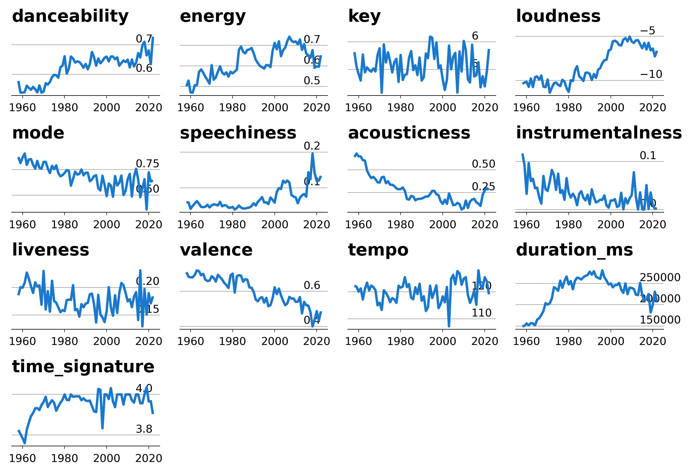
There are some clear features that have changed over time:
Danceability (0-1): Danceability describes how suitable a track is for dancing based on a combination of musical elements including tempo, rhythm stability, beat strength, and overall regularity.
Energy (0-1): Typically, energetic tracks feel fast, loud, and noisy. For example, death metal has high energy, while a Bach prelude scores low on the scale. Perceptual features contributing to this attribute include dynamic range, perceived loudness, timbre, onset rate, and general entropy.
Loudness: The overall loudness of a track in decibels (dB). Loudness values are averaged across the entire track and are useful for comparing relative loudness of tracks.
Mode: Mode indicates the modality (major or minor) of a track, the type of scale from which its melodic content is derived.
Speechiness (0-1): Speechiness detects the presence of spoken words in a track. The more exclusively speech-like the recording (e.g. talk show, audio book, poetry), the closer to 1.0 the attribute value.
Acousticness: A confidence measure from 0.0 to 1.0 of whether the track is acoustic. 1.0 represents high confidence the track is acoustic.
Duration: The duration of the track in milliseconds.
Valence: A measure from 0.0 to 1.0 describing the musical positiveness conveyed by a track. Tracks with high valence sound more positive (e.g. happy, cheerful, euphoric), while tracks with low valence sound more negative (e.g. sad, depressed, angry).
Duration
fig, ax = plt.subplots()
ax.plot(year['year'], (year['duration_ms'] / 1_000) / 60)
ax.set_xlim(1958, 2026)
ax.set_ylim(0,6.5)

# Add in title and subtitle
ax.set_title("""Ain't nobody got time for that""")
ax.text(x=.08, y=.86,
        s="Average duration in minutes. Features from top ten singles, 1958-2022.",
        transform=fig.transFigure,
        ha='left',
        fontsize=20,
        alpha=.8)

# Set the logo
logo = plt.imread('images/datafantic.png')
imagebox = OffsetImage(logo, zoom=.22)
ab = AnnotationBbox(imagebox, xy=(1,1.06), xycoords='axes fraction', box_alignment=(1,1), frameon = False)
ax.add_artist(ab)


# Export plot as high resolution PNG
plt.savefig('images/music_features_duration.png')
Loudness
fig, ax = plt.subplots()
ax.plot(year['year'], year['loudness'])
ax.set_xlim(1958, 2026)
ax.set_ylim(-15, -3)

# Add in title and subtitle
ax.set_title("""Hearing protection recommended""")
ax.text(x=.08, y=.86,
        s="Average loudness in decibels (-60-0). Features from top ten singles, 1958-2022.",
        transform=fig.transFigure,
        ha='left',
        fontsize=20,
        alpha=.8)

# Set the logo
logo = plt.imread('images/datafantic.png')
imagebox = OffsetImage(logo, zoom=.22)
ab = AnnotationBbox(imagebox, xy=(1,1.06), xycoords='axes fraction', box_alignment=(1,1), frameon = False)
ax.add_artist(ab)


# Export plot as high resolution PNG
plt.savefig('images/music_features_loudness.png')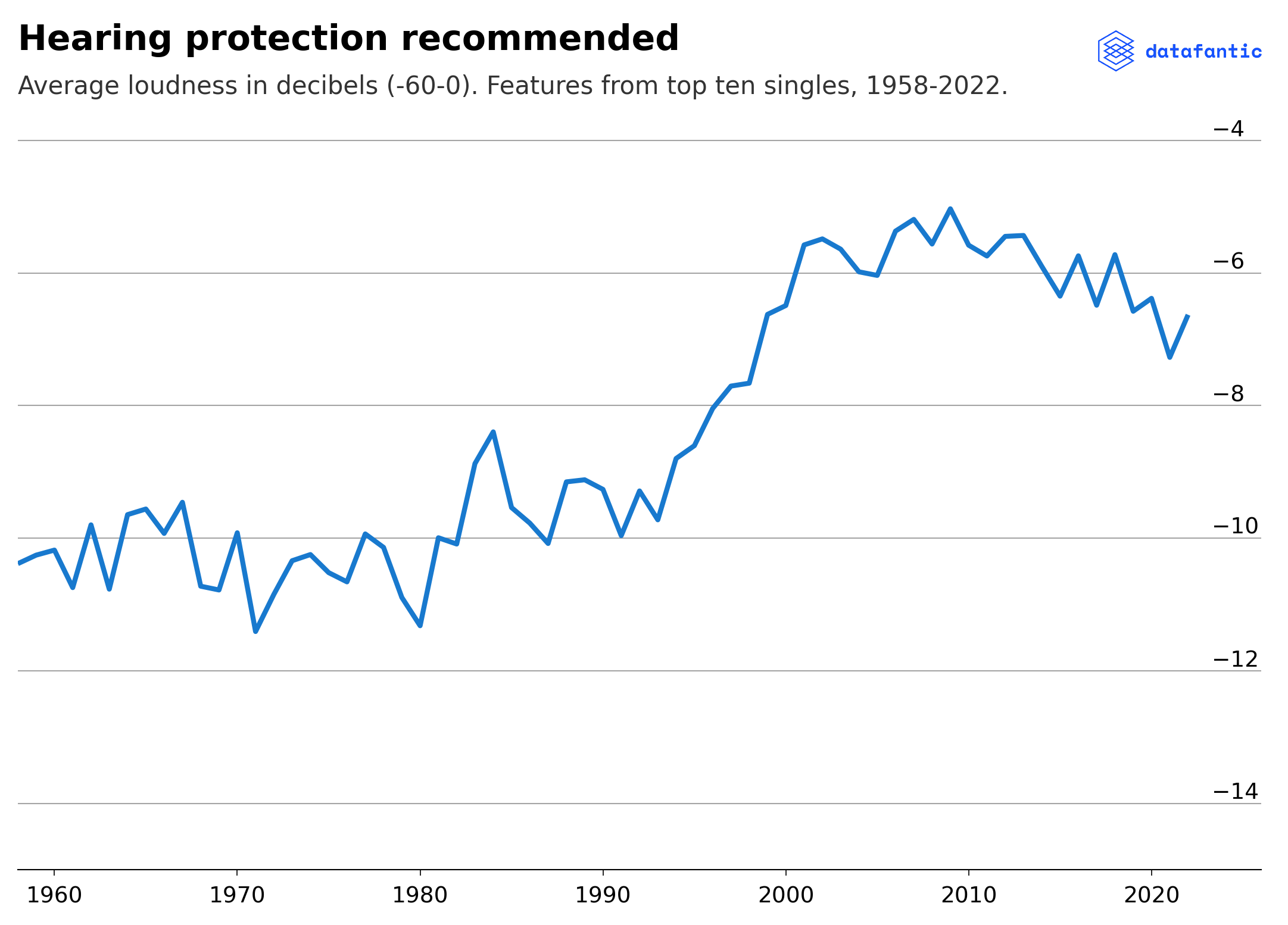
Features Trending Down
The features that are trending down:
Valence
Instrumentalness (shown separately)
Acousticness
fig, ax = plt.subplots()
ax.plot(year['year'], year['valence'])
ax.plot(year['year'], year['acousticness'])
ax.set_xlim(1958, 2025)
ax.set_ylim(0,.85)

# Add in title and subtitle
ax.set_title("""I've got a negative feeling""")
ax.text(x=.08, y=.86,
        s="Average features from top ten singles, 1958-2022, Scale 0-1",
        transform=fig.transFigure,
        ha='left',
        fontsize=20,
        alpha=.8)

# Label the lines directly
ax.text(x=.78, y=.66, s="""Valence""",
        transform=fig.transFigure, ha='left', fontsize=20, alpha=.7)
ax.text(x=.73, y=.30, s="""Acousticness""",
        transform=fig.transFigure, ha='left', fontsize=20, alpha=.7)

# Set the logo
logo = plt.imread('images/datafantic.png')
imagebox = OffsetImage(logo, zoom=.22)
ab = AnnotationBbox(imagebox, xy=(1,1.06), xycoords='axes fraction', box_alignment=(1,1), frameon = False)
ax.add_artist(ab)


# Export plot as high resolution PNG
plt.savefig('images/music_features_trending_down.png')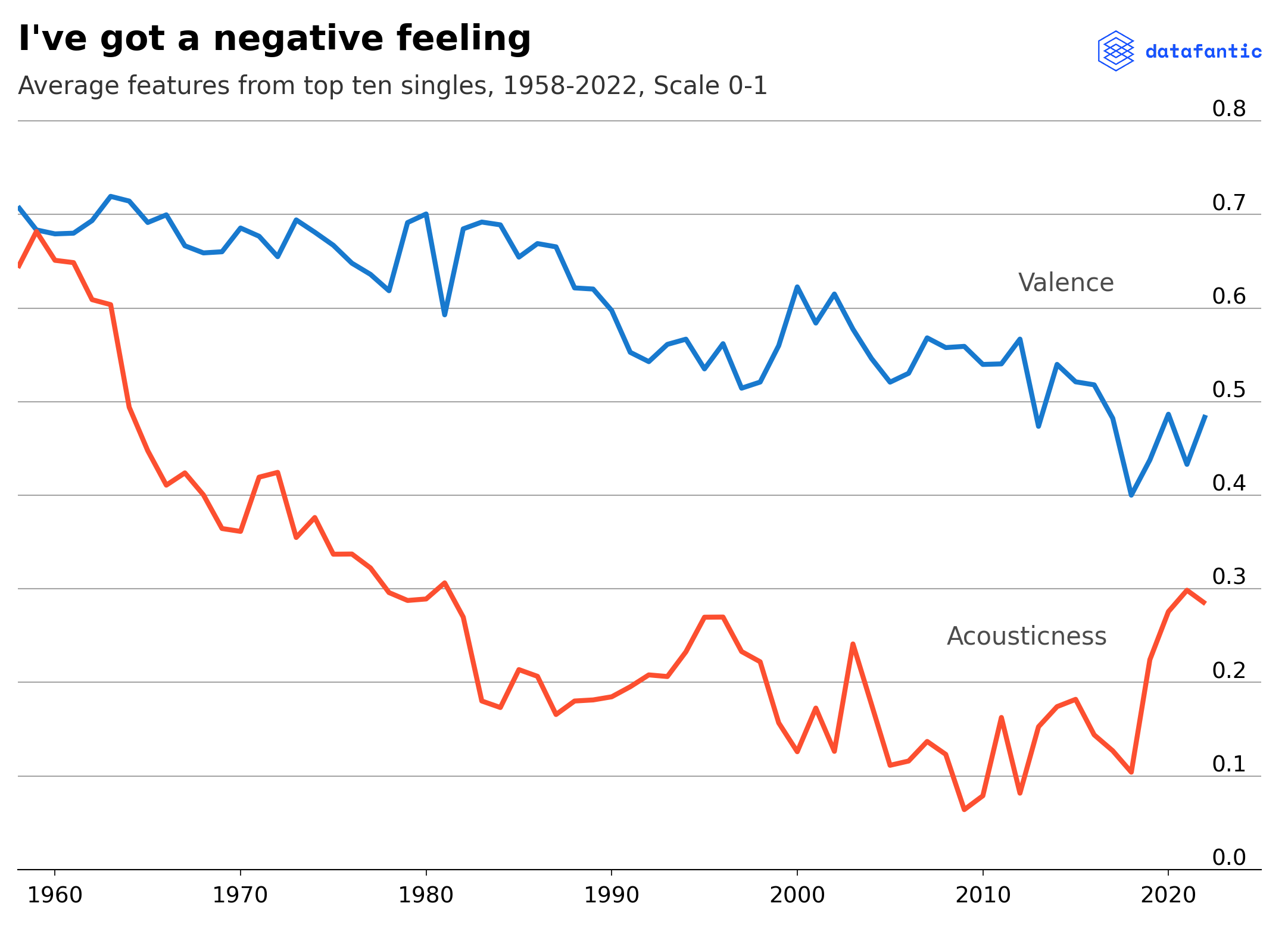
Features Trending Up
Danceability
Energy
Speechiness (shown below)
fig, ax = plt.subplots()
ax.plot(year['year'], year['danceability'])
ax.plot(year['year'], year['energy'])
ax.set_xlim(1958, 2025)
ax.set_ylim(0,.85)

# Add in title and subtitle
ax.set_title('>10% more danceability')
ax.text(x=.08, y=.86,
        s="Average features from top ten singles, 1958-2022, Scale 0-1",
        transform=fig.transFigure,
        ha='left',
        fontsize=20,
        alpha=.8)

# Label the lines directly
ax.text(x=.7, y=.795, s="""Energy""",
        transform=fig.transFigure, ha='left', fontsize=20, alpha=.7)
ax.text(x=.685, y=.61, s="""Danceability""",
        transform=fig.transFigure, ha='left', fontsize=20, alpha=.7)

# Set the logo
logo = plt.imread('images/datafantic.png')
imagebox = OffsetImage(logo, zoom=.22)
ab = AnnotationBbox(imagebox, xy=(1,1.06), xycoords='axes fraction', box_alignment=(1,1), frameon = False)
ax.add_artist(ab)


# Export plot as high resolution PNG
plt.savefig('images/music_features_trending_up.png')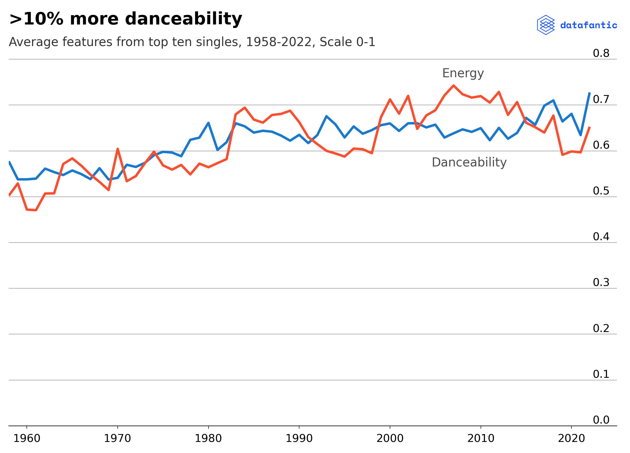
Speechiness vs Instrumentalness
fig, ax = plt.subplots()
ax.plot(year['year'], year['instrumentalness'])
ax.plot(year['year'], year['speechiness'])
ax.set_xlim(1958, 2025)
ax.set_ylim(0,.32)

ax.set_yticks(np.arange(0, .35, 0.05))

# Add in title and subtitle
ax.set_title("They don't sing like they used to..")
ax.text(x=.08, y=.86,
        s="Average features from top ten singles, 1958-2022, Scale 0-1",
        transform=fig.transFigure,
        ha='left',
        fontsize=20,
        alpha=.8)

# Label the lines directly
ax.text(x=.57, y=.17, s="""Instrumentalness""",
        transform=fig.transFigure, ha='left', fontsize=20, alpha=.7)
ax.text(x=.72, y=.52, s="""Speechiness""",
        transform=fig.transFigure, ha='left', fontsize=20, alpha=.7)

# Set the logo
logo = plt.imread('images/datafantic.png')
imagebox = OffsetImage(logo, zoom=.22)
ab = AnnotationBbox(imagebox, xy=(1,1.06), xycoords='axes fraction', box_alignment=(1,1), frameon = False)
ax.add_artist(ab)


# Export plot as high resolution PNG
plt.savefig('images/music_features_instrumentalness_speechiness.png')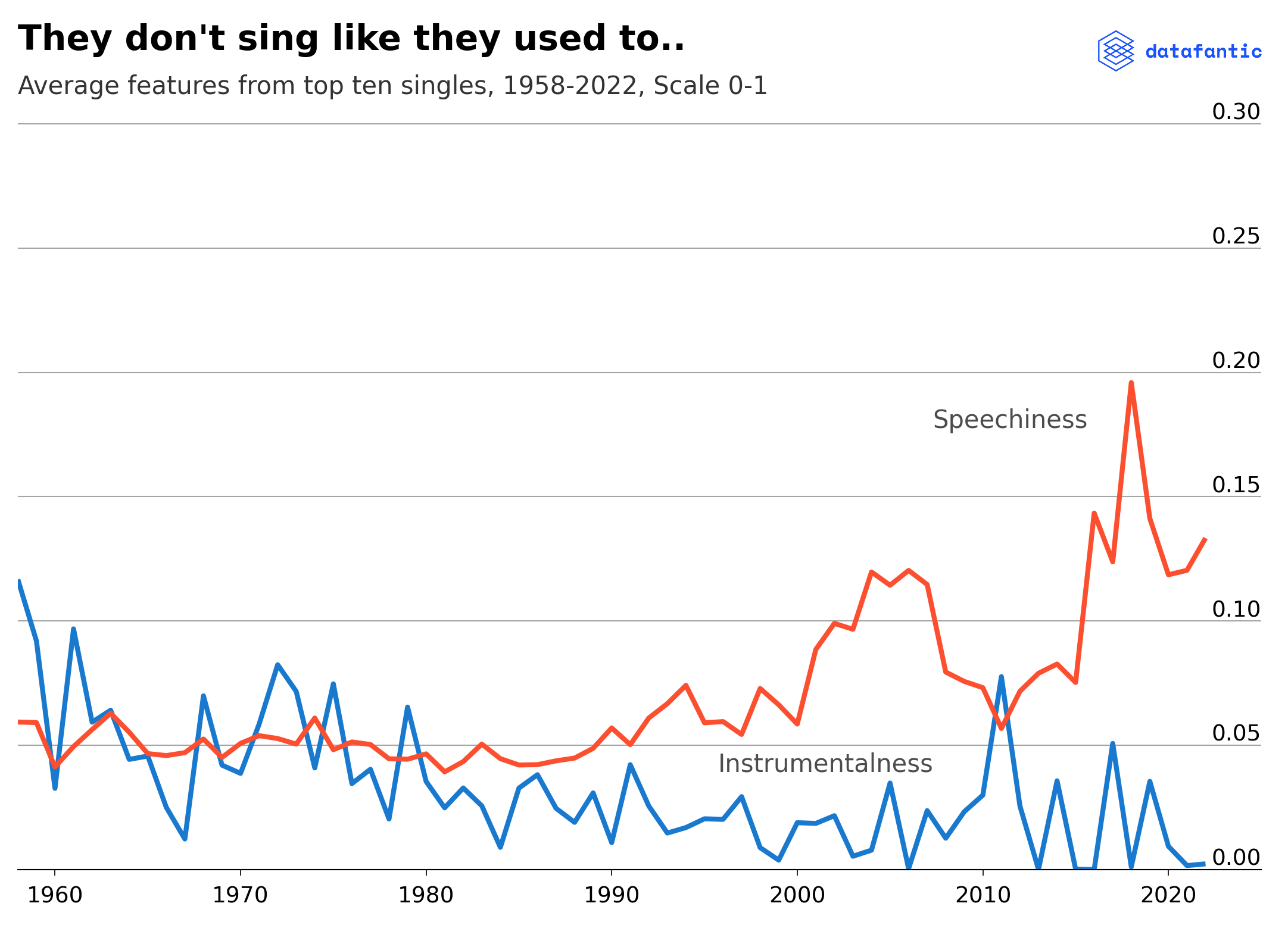
 Created in