Whopper Index

This notebook takes the raw Whopper prices in local currency and the USD exchange rate to calculate the Whopper Index.

To calculate the Whopper Index, we first calculate the implied exchange rate based on the Whopper price locally and in the US. For example:

In the Czech Republic, a Whopper costs 99 Czech Korunas.
In the US, a Whopper costs $6.09 USD.
The implied exchange rate is 99 CZK/USD, which is 99CZK/$6.09USD = 16.25.

From there, we can compare this to the actual exchange rate to see if the currency is over or under-valued. For example:

The implied exchange rate according to the Whopper index is 16.25 CZK/USD
The actual exchange rate is 24.61 CZK/USD.
We can find the currency over/undervaluation between the two by taking: (Implied FX Rate - Actual FX Rate) / Actual FX Rate. (16.25 - 24.61) / 24.61 = -33.9% undervalued

Now let’s import our data and calculate the index.

import pandas as pd
import numpy as np

import matplotlib.pyplot as plt
from matplotlib.offsetbox import (OffsetImage, AnnotationBbox)

df = pd.read_csv('data/whopper_prices.csv')
df.sample(5)

	date	iso_a3	currency_code	currency_name	name	local_price	dollar_ex
14	9/1/2022	HUN	HUF	Forint	Hungary	1590.0	396.42
39	9/1/2022	KOR	KRW	Won	South Korea	6400.0	1381.00
15	9/1/2022	IND	INR	Indian Rupee	India	299.0	79.70
1	9/1/2022	AUS	AUD	Australian Dollar	Australia	9.4	1.48
16	9/1/2022	IDN	IDR	Rupiah	Indonesia	54545.0	14890.02

df.shape

(49, 7)

Countries not on the Big Mac Index

Our data contains local prices and USD exchange rates for 50 countries. Notably there are several countries on our list that are not contained in the Big Mac Index.

big_mac = pd.read_csv('data/big-mac-raw-index.csv')

big_mac_countries = list(big_mac[big_mac['date'] == '2022-01-01']['iso_a3'])
whopper_countries = list(df['iso_a3'])

We can see that there are 9 countries on our Whopper list that are not on the Big Mac Index. These include two countries in Central Asia and 3 countries in Africa.

extra_countries = list(set(whopper_countries).difference(big_mac_countries))
extra_countries

['MNG', 'NGA', 'KAZ', 'BGD', 'KEN', 'MAR', 'MDV', 'IRQ', 'BLR']

df[df['iso_a3'].isin(extra_countries)]['name']

3     Bangladesh
4        Belarus
17          Iraq
20    Kazakhstan
21         Kenya
23      Maldives
24      Mongolia
25       Morocco
28       Nigeria
Name: name, dtype: object

big_mac_2022 = big_mac[big_mac['date'] == '2022-07-01']

big_mac_2022[big_mac_2022['iso_a3'].isin(list(set(big_mac_countries).difference(whopper_countries)))]['name']

1580                 Bahrain
1584                   Chile
1585                   China
1586                Colombia
1587              Costa Rica
1593                Honduras
1600                  Jordan
1602                 Lebanon
1603                Malaysia
1604                  Mexico
1605                 Moldova
1609                    Oman
1615                 Romania
1620               Sri Lanka
1626    United Arab Emirates
1629               Venezuela
Name: name, dtype: object

Build Index

Now we can move forward and build the index. First we will calculate the local price in USD at the current exchange. This will help us build a sense of “How many Whoppers can I buy with $50 USD?”. This is one of the halmarks of the Economist’s Big Mac index, and a very easy way to understand purchasing power parity.

Then we will calculate the implied exchange rate and finally the index.

us_price = df[df['iso_a3'] == 'USA']['local_price'].iat[0]

df = (df.assign(dollar_price = lambda x: x['local_price'] / x['dollar_ex'],
                implied_ex = lambda x: x['local_price'] / us_price,
                usd_index = lambda x: round(((x['implied_ex'] - x['dollar_ex']) / x['dollar_ex']) * 100, 2))
        .sort_values(by='usd_index', ignore_index=True)
    )

df

	date	iso_a3	currency_code	currency_name	name	local_price	dollar_ex	dollar_price	implied_ex	usd_index
0	9/1/2022	ZAF	ZAR	Rand	South Africa	29.90	17.300	1.728324	4.909688	-71.62
1	9/1/2022	PAK	PKR	Pakistan Rupee	Pakistan	540.00	222.740	2.424351	88.669951	-60.19
2	9/1/2022	PHL	PHP	Philippine Peso	Philippines	177.00	57.180	3.095488	29.064039	-49.17
3	9/1/2022	BLR	BYN	Belarussian Ruble	Belarus	7.90	2.520	3.134921	1.297209	-48.52
4	9/1/2022	PER	PEN	Neuvo Sol	Peru	12.90	3.890	3.316195	2.118227	-45.55
5	9/1/2022	MNG	MNT	Tugrik	Mongolia	10900.00	3227.000	3.377750	1789.819376	-44.54
6	9/1/2022	EGY	EGP	Egyptian Pound	Egypt	66.00	19.260	3.426791	10.837438	-43.73
7	9/1/2022	QAT	QAR	Qatari Rial	Qatar	13.00	3.640	3.571429	2.134647	-41.36
8	9/1/2022	IDN	IDR	Rupiah	Indonesia	54545.00	14890.020	3.663192	8956.486043	-39.85
9	9/1/2022	GTM	GTQ	Quetzal	Guatemala	29.00	7.750	3.741935	4.761905	-38.56
10	9/1/2022	IND	INR	Indian Rupee	India	299.00	79.700	3.751568	49.096880	-38.40
11	9/1/2022	TUR	TRY	Turkish Lira	Turkey	69.00	18.240	3.782895	11.330049	-37.88
12	9/1/2022	POL	PLN	Zloty	Poland	17.99	4.710	3.819533	2.954023	-37.28
13	9/1/2022	RUS	RUB	Russian Ruble	Russia	239.99	62.450	3.842914	39.407225	-36.90
14	9/1/2022	HRV	HRK	Kuna	Croatia	29.00	7.520	3.856383	4.761905	-36.68
15	9/1/2022	TWN	TWD	New Taiwan Dollar	Taiwan	123.00	30.910	3.979295	20.197044	-34.66
16	9/1/2022	HUN	HUF	Forint	Hungary	1590.00	396.420	4.010898	261.083744	-34.14
17	9/1/2022	CZE	CZK	Czech Koruna	Czech Republic	99.00	24.610	4.022755	16.256158	-33.94
18	9/1/2022	AZE	AZN	Azerbaijanian Manat	Azerbaijan	6.90	1.700	4.058824	1.133005	-33.35
19	9/1/2022	URY	UYU	Peso Uruguayo	Uruguay	169.00	40.390	4.184204	27.750411	-31.29
20	9/1/2022	KAZ	KZT	Tenge	Kazakhstan	2000.00	473.860	4.220656	328.407225	-30.70
21	9/1/2022	KWT	KWD	Kuwaiti Dinar	Kuwait	1.40	0.309	4.530744	0.229885	-25.60
22	9/1/2022	BGD	BDT	Taka	Bangladesh	439.00	95.060	4.618136	72.085386	-24.17
23	9/1/2022	KOR	KRW	Won	South Korea	6400.00	1381.000	4.634323	1050.903120	-23.90
24	9/1/2022	SGP	SGD	Singapore Dollar	Singapore	6.70	1.400	4.785714	1.100164	-21.42
25	9/1/2022	JPN	JPY	Yen	Japan	690.00	144.090	4.788674	113.300493	-21.37
26	9/1/2022	VNM	VND	Dong	Vietnam	115000.00	23702.000	4.851911	18883.415435	-20.33
27	9/1/2022	KEN	KES	Kenyan Shilling	Kenya	590.00	120.340	4.902775	96.880131	-19.49
28	9/1/2022	MAR	MAD	Moroccan Dirham	Morocco	52.00	10.590	4.910293	8.538588	-19.37
29	9/1/2022	NIC	NIO	Cordoba Oro	Nicaragua	176.00	35.700	4.929972	28.899836	-19.05
30	9/1/2022	BRA	BRL	Brazilian Real	Brazil	26.90	5.240	5.133588	4.417077	-15.70
31	9/1/2022	IRQ	IQD	Iraqi Dinar	Iraq	7500.00	1459.430	5.138993	1231.527094	-15.62
32	9/1/2022	THA	THB	Baht	Thailand	189.00	36.420	5.189456	31.034483	-14.79
33	9/1/2022	CAN	CAD	Canadian Dollar	Canada	7.39	1.310	5.641221	1.213465	-7.37
34	9/1/2022	GBR	GBP	Pound Sterling	United Kingdom	4.99	0.860	5.802326	0.819376	-4.72
35	9/1/2022	EUZ	EUR	Euro	Euro Area	5.82	1.000	5.820000	0.955665	-4.43
36	9/1/2022	ARG	ARS	Argentine Peso	Argentina	850.00	140.740	6.039505	139.573071	-0.83
37	9/1/2022	USA	USD	US Dollar	United States	6.09	1.000	6.090000	1.000000	0.00
38	9/1/2022	AUS	AUD	Australian Dollar	Australia	9.40	1.480	6.351351	1.543514	4.29
39	9/1/2022	SAU	SAR	Saudi Riyal	Saudi Arabia	25.00	3.750	6.666667	4.105090	9.47
40	9/1/2022	NZL	NZD	New Zealand Dollar	New Zealand	11.00	1.650	6.666667	1.806240	9.47
41	9/1/2022	MDV	MVR	Rufiyaa	Maldives	105.00	15.320	6.853786	17.241379	12.54
42	9/1/2022	NGA	NGN	Naira	Nigeria	3000.00	426.100	7.040601	492.610837	15.61
43	9/1/2022	HKG	HKD	Hong Kong Dollar	Hong Kong	59.00	7.840	7.525510	9.688013	23.57
44	9/1/2022	SWE	SEK	Swedish Krona	Sweden	85.00	10.720	7.929104	13.957307	30.20
45	9/1/2022	NOR	NOK	Norwegian Krone	Norway	83.00	10.010	8.291708	13.628900	36.15
46	9/1/2022	ISR	ILS	New Israeli Sheqel	Israel	29.00	3.420	8.479532	4.761905	39.24
47	9/1/2022	CHE	CHF	Swiss Franc	Switzerland	8.40	0.977	8.597748	1.379310	41.18
48	9/1/2022	DNK	DKK	Danish Krone	Denmark	67.00	7.440	9.005376	11.001642	47.87

df.to_csv("data/whopper_index.csv", index=False)

Plot Index

plt.style.use("datafantic.mplstyle")

fig, ax = plt.subplots(figsize=(9, 18))
ax.barh(df['name'], df['usd_index'], height=0.7, linewidth=1)

# Add horizontal line where the US is
ax.axhline(37, color='black', linewidth=1)

# Move x axis to top and change tick labels
ax.xaxis.tick_top()
ax.tick_params(axis='x', 
               which='major', 
               labelsize=16, 
               top=False, 
               pad=1)
ax.set_xticks(np.arange(-60, 60, 20), labels=['-60%', '-40','-20','0', '20', '40%'])

ax.set_xlabel("                 <-- Undervalued              Overvalued -->", 
              labelpad=10, 
              fontsize=16)
ax.xaxis.set_label_position('top') 

# Change grid and font sizes
ax.grid(False)
ax.grid(True, which='major', axis='x')
ax.spines.bottom.set_visible(False)

# Shrink y axis
ax.set_ylim(-1, df.shape[0])

# Add in title and subtitle
ax.text(x=-0.15, y=.93, 
        s="The Whopper Index", 
        transform=fig.transFigure, 
        ha='left', 
        fontsize=28, 
        fontweight='bold')
        

# Set the logo
logo = plt.imread('images/datafantic.png')
imagebox = OffsetImage(logo, zoom=.22)
ab = AnnotationBbox(imagebox, 
                    xy=(1,1.1), 
                    xycoords='axes fraction', 
                    box_alignment=(1,1), 
                    frameon = False)
ax.add_artist(ab)


# Export plot as high resolution PNG
plt.savefig('images/whopper_index.png')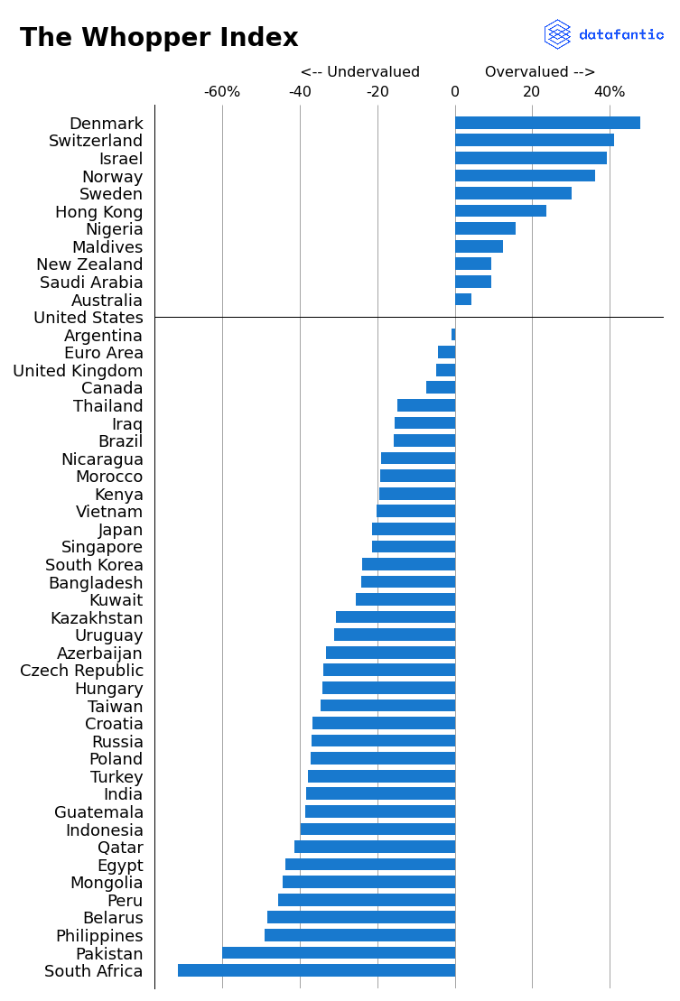

Compare to Big Mac Index

The Big Mac Index isn’t a perfect measure of PPP, and neither is our Whopper Index. However, by comparing them we might find useful differences to interpret. We will plot the

big_mac = big_mac.rename(columns={'dollar_price':'big_mac_dollar_price'})

compare = (df.merge(big_mac[big_mac['date'] == '2022-07-01'][['iso_a3','USD','big_mac_dollar_price']], how='left', on='iso_a3')
             .rename(columns={'USD':'big_mac_index'})
             .dropna()
             .reset_index(drop=True)
             .assign(big_mac_index = lambda x: round(x['big_mac_index'] * 100, 2))
)

compare.head()

	date	iso_a3	currency_code	currency_name	name	local_price	dollar_ex	dollar_price	implied_ex	usd_index	big_mac_index	big_mac_dollar_price
0	9/1/2022	ZAF	ZAR	Rand	South Africa	29.9	17.30	1.728324	4.909688	-71.62	-54.52	2.342065
1	9/1/2022	PAK	PKR	Pakistan Rupee	Pakistan	540.0	222.74	2.424351	88.669951	-60.19	-38.70	3.156708
2	9/1/2022	PHL	PHP	Philippine Peso	Philippines	177.0	57.18	3.095488	29.064039	-49.17	-46.51	2.754821
3	9/1/2022	PER	PEN	Neuvo Sol	Peru	12.9	3.89	3.316195	2.118227	-45.55	-30.67	3.570649
4	9/1/2022	EGY	EGP	Egyptian Pound	Egypt	66.0	19.26	3.426791	10.837438	-43.73	-52.85	2.428081

fig, ax = plt.subplots(figsize=(9, 18))
ax.barh(compare['name'], compare['usd_index'], height=0.7, linewidth=1, zorder=1)

# Add in Big Mac Index data
ax.hlines(y=compare.index, 
          xmin=[0] * compare.shape[0], 
          xmax=compare['big_mac_index'], 
          color='#FC4F30', 
          zorder=2, 
          linewidth=1, 
          label='_nolegend_')
ax.scatter(compare['big_mac_index'], np.arange(compare.shape[0]), s=50, zorder=3)


# Add horizontal line where the US is
ax.axhline(29, color='black', linewidth=1)

# Move x axis to top and change tick labels
ax.xaxis.tick_top()
ax.tick_params(axis='x', 
               which='major', 
               labelsize=16, 
               top=False, 
               pad=1)
ax.set_xticks(np.arange(-60, 60, 20), labels=['-60%', '-40','-20','0', '20', '40%'])

ax.set_xlabel("                       <-- Undervalued              Overvalued -->", 
              labelpad=10, 
              fontsize=16)
ax.xaxis.set_label_position('top') 

# Change grid and font sizes
ax.grid(False)
ax.grid(True, which='major', axis='x')
ax.spines.bottom.set_visible(False)

# Shrink y axis
ax.set_ylim(-1, compare.shape[0])

# Add in title and subtitle
ax.text(x=-0.15, y=.95, 
        s="Double Burger Index", 
        transform=fig.transFigure, 
        ha='left', 
        fontsize=28, 
        fontweight='bold')
ax.text(x=-0.15, y=.93, 
        s="Comparison of Big Mac (red) and Whopper Index (blue)", 
        transform=fig.transFigure, 
        ha='left', 
        fontsize=20, 
        alpha=0.8)
        

# Set the logo
logo = plt.imread('images/datafantic.png')
imagebox = OffsetImage(logo, zoom=.22)
ab = AnnotationBbox(imagebox, 
                    xy=(1,1.12), 
                    xycoords='axes fraction', 
                    box_alignment=(1,1), 
                    frameon = False)
ax.add_artist(ab)


# Export plot as high resolution PNG
plt.savefig('images/index_comparison.png')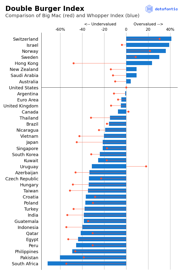

Comparing Whopper and Big Mac Prices

My wife (a very smart lady), brought an idea to my attention. While these indices are comparable, we can also compare the price of Big Macs and Whoppers directly. My main concern here is that the prices I’m collecting often come from delivery services. This might be skewing things enough to cause problems.

fig, ax = plt.subplots(figsize=(9, 18))
bar1 = ax.barh(compare['name'], compare['dollar_price'].round(2), height=0.7, linewidth=1, zorder=1)
bar2 = ax.barh(compare['name'], -compare['big_mac_dollar_price'].round(2), height=0.7, linewidth=1, zorder=1)

ax.bar_label(bar1, padding=5, fmt='$%.2f', fontsize=16)
ax.bar_label(bar2, padding=5, labels=['$%.2f' % np.absolute(e) for e in compare['big_mac_dollar_price']], fontsize=16)

# Move x axis to top and change tick labels
plt.tick_params(
    axis='x',
    which='both',
    bottom=False,
    top=False,
    labelbottom=False)

# Change grid and font sizes
ax.grid(False)
ax.grid(True, which='major', axis='x')
ax.spines.bottom.set_visible(False)

# Shrink y axis and expand x axis
ax.set_ylim(-1, compare.shape[0])
ax.set_xlim(-10, 9)

# Change grid and font sizes
ax.grid(False)
ax.spines.bottom.set_visible(False)

# Add in title and subtitle
ax.text(x=-0.15, y=.95, 
        s="Burgernomics", 
        transform=fig.transFigure, 
        ha='left', 
        fontsize=28, 
        fontweight='bold')
ax.text(x=-0.15, y=.93, 
        s="Big Mac and Whopper Prices around the world in USD", 
        transform=fig.transFigure, 
        ha='left', 
        fontsize=20, 
        alpha=0.8)

# Add McDonalds and Burger King Logo
bk_logo = plt.imread('images/burger_king_logo.png')
imagebox = OffsetImage(bk_logo, zoom=.12)
ab = AnnotationBbox(imagebox, 
                    xy=(.8,1.046), 
                    xycoords='axes fraction', 
                    box_alignment=(1,1), 
                    frameon = False)
ax.add_artist(ab)

mc_logo = plt.imread('images/mcdonalds_logo.png')
imagebox = OffsetImage(mc_logo, zoom=.03)
ab = AnnotationBbox(imagebox, 
                    xy=(.45,1.04), 
                    xycoords='axes fraction', 
                    box_alignment=(1,1), 
                    frameon = False)
ax.add_artist(ab)

# Set the logo
logo = plt.imread('images/datafantic.png')
imagebox = OffsetImage(logo, zoom=.22)
ab = AnnotationBbox(imagebox, 
                    xy=(1,1.12), 
                    xycoords='axes fraction', 
                    box_alignment=(1,1), 
                    frameon = False)
ax.add_artist(ab)

# Set source text
ax.text(x=-0.15, y=0.1, 
        s="""Source: The Economist, datafantic""", 
        transform=fig.transFigure, 
        ha='left', 
        fontsize=12, 
        alpha=.7)



# Export plot as high resolution PNG
plt.savefig('images/price_comparison.png')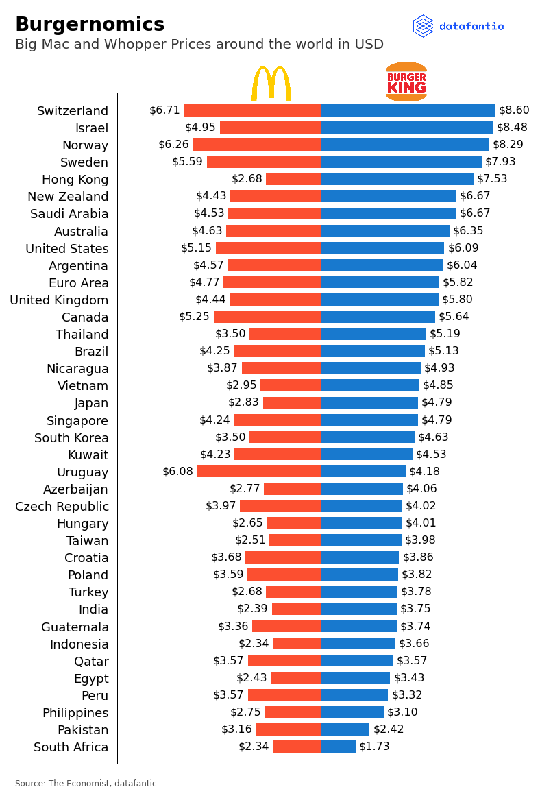

Most Expensive Whoppers

Let’s take a look at the most expensive Whoppers.

fig, ax = plt.subplots(figsize=(14, 11))
bar1 = ax.barh(df['name'][-10:], df['dollar_price'][-10:].round(2), height=0.7, linewidth=1, zorder=1)
ax.bar_label(bar1, padding=5, fmt='$%.2f', fontsize=18)

# Add horizontal line where the US is
ax.axhline(29, color='black', linewidth=1)

# Move x axis to top and change tick labels
plt.tick_params(
    axis='x',
    which='both',
    bottom=False,
    top=False,
    labelbottom=False)

# Shrink y axis
ax.set_ylim(-1, df[-10:].shape[0])
ax.set_xlim(5, 9.1)

# Change grid and font sizes
ax.grid(False)
ax.spines.bottom.set_visible(False)
ax.spines.left.set_visible(False)

# Add in title and subtitle
ax.text(x=-0.04, y=.9, 
        s="Whopping Prices", 
        transform=fig.transFigure, 
        ha='left', 
        fontsize=28, 
        fontweight='bold')
ax.text(x=-0.04, y=.86, 
        s="Top 10 country Whopper prices in USD, from the Whopper Index", 
        transform=fig.transFigure, 
        ha='left', 
        fontsize=20, 
        alpha=.8)

# Set the logo
logo = plt.imread('images/datafantic.png')
imagebox = OffsetImage(logo, zoom=.22)
ab = AnnotationBbox(imagebox, xy=(1.01,1.06), xycoords='axes fraction', box_alignment=(1,1), frameon = False)
ax.add_artist(ab)

# Export plot as high resolution PNG
plt.savefig('images/top_whopper_prices.png')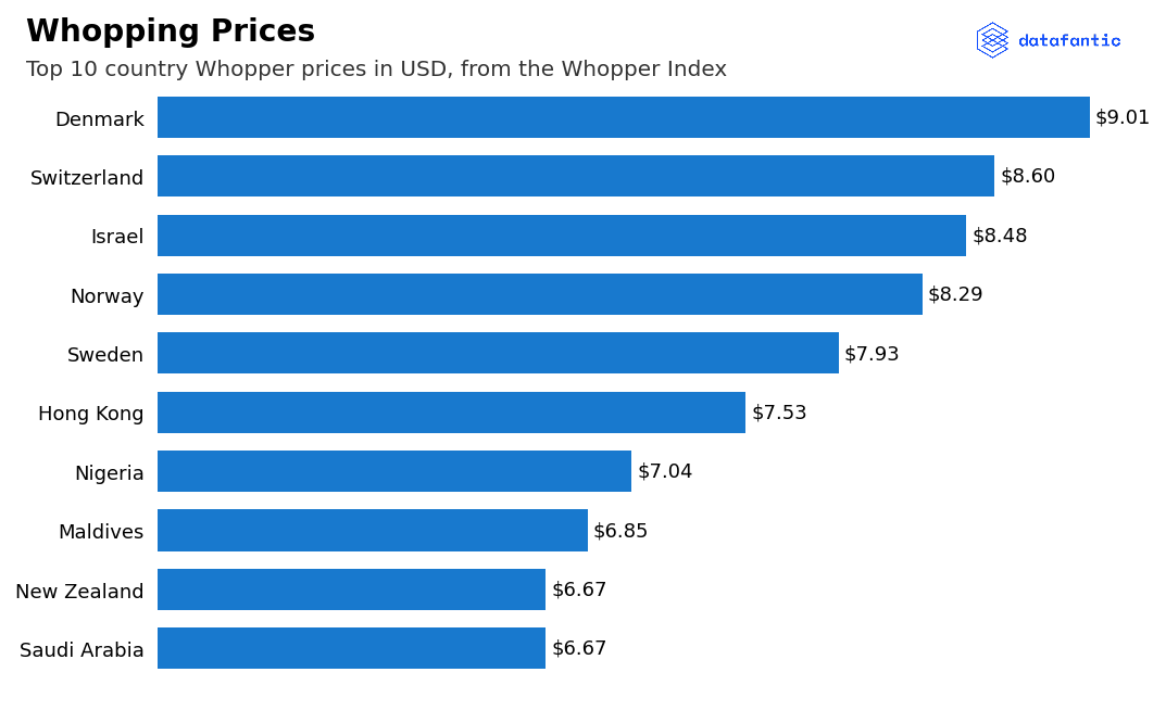

Now let’s look at the cheapest Whoppers

fig, ax = plt.subplots(figsize=(14, 11))
bar1 = ax.barh(df['name'][:10], df['dollar_price'][:10], height=0.7, linewidth=1, zorder=1)
ax.bar_label(bar1, padding=5, fmt='$%.2f', fontsize=18)

# Add horizontal line where the US is
ax.axhline(29, color='black', linewidth=1)

# Move x axis to top and change tick labels
plt.tick_params(
    axis='x',
    which='both',
    bottom=False,
    top=False,
    labelbottom=False)

# Shrink y axis
ax.set_ylim(-1, df[:10].shape[0])
ax.set_xlim(1, 3.9)

# Change grid and font sizes
ax.grid(False)
ax.spines.bottom.set_visible(False)
ax.spines.left.set_visible(False)

# Add in title and subtitle
ax.text(x=-0.04, y=.9, 
        s="Whopping Value", 
        transform=fig.transFigure, 
        ha='left', 
        fontsize=28, 
        fontweight='bold')
ax.text(x=-0.04, y=.86, 
        s="Lowest 10 country Whopper prices in USD, from the Whopper Index", 
        transform=fig.transFigure, 
        ha='left', 
        fontsize=20, 
        alpha=.8)

# Set the logo
logo = plt.imread('images/datafantic.png')
imagebox = OffsetImage(logo, zoom=.22)
ab = AnnotationBbox(imagebox, xy=(1.01,1.06), xycoords='axes fraction', box_alignment=(1,1), frameon = False)
ax.add_artist(ab)

# Export plot as high resolution PNG
plt.savefig('images/bottom_whopper_prices.png')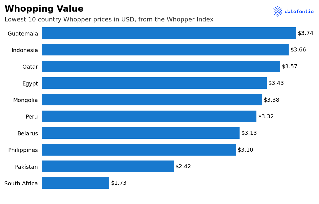

Created in deepnote.com Created in Deepnote